[2]:
import torch
import numpy as np
import matplotlib.pyplot as plt
import numpy as np

from svetlanna.phase_retrieval_problem import phase_retrieval
from svetlanna import SimulationParameters
from svetlanna import Wavefront
from svetlanna import elements
from svetlanna import LinearOpticalSetup
from svetlanna.units import ureg
Phase retrieval problem
Consider an optical system consisting of a source generating a Gaussian beam, a collecting lens, and a screen located in the rear focal plane of the lens.
First, let us solve the forward problem and see what intensity distribution will be obtained if a beam passes through such a system. Then let us solve the inverse problem using svetlanna.phase_retrieval module: knowing the intensity distribution on the screen after the passage of the optical system described above and the intensity distribution in the plane after the lens, let us try to find the transmission function of the lens
Creating numerical mesh with using SimulationParameters class
[188]:
# optical setup size
lx = 10 * ureg.mm
ly = 10 * ureg.mm

# number of nodes
Nx = 1024
Ny = 1024

# wavelength
wavelength = 1064 * ureg.nm

# focal distance of the lens
focal = 10 * ureg.cm
# radius of the lens
r = 1 * ureg.cm
# distance between the screen and the lens
distance = focal * 1.

# waist radius of the gaussian beam
w0 = 1 * ureg.mm

# creating SimulationParameters exemplar
sim_params = SimulationParameters({
    'W': torch.linspace(-lx / 2, lx / 2, Nx),
    'H': torch.linspace(-ly / 2, ly / 2, Ny),
    'wavelength': wavelength,
})
[189]:
# return 2d-tensors of x and y coordinates
x_grid, y_grid = sim_params.meshgrid(x_axis='W', y_axis='H')
Solving a direct problem
[190]:
incident_wavefront = Wavefront.gaussian_beam(
    simulation_parameters=sim_params,
    waist_radius=w0,
    distance=distance
)

source_intensity = incident_wavefront.intensity

lens = elements.ThinLens(
    simulation_parameters=sim_params,
    focal_length=focal,
    radius=r
)

field_after_lens = lens.forward(incident_wavefront=incident_wavefront)

free_space = elements.FreeSpace(
    simulation_parameters=sim_params,
    distance=distance,
    method="AS"
)

output_field = free_space.forward(incident_wavefront=field_after_lens)

target_intensity = output_field.intensity
Creating optical setup that describes field propagation from source to the screen
[191]:
optical_setup = LinearOpticalSetup([free_space])
Solving phase retrieval problem
In order to solve the phase retrieval problem it’s necessary to define the source_intensity, target_intensity and optimization method in phase_retrieval.retrieve_phase function. Optionally, you can define algorithm’s parameters using options parameter. You must pass the dict with key arguments
[192]:
result_gs = phase_retrieval.retrieve_phase(
    source_intensity=source_intensity,
    optical_setup=optical_setup,
    target_intensity=target_intensity,
    method='GS',
    options= {
        'tol': 1e-16,
        'maxiter': 12,
        'disp': False
    }
)
[193]:
phase_distribution_gs = result_gs.solution
niter_gs = result_gs.number_of_iterations
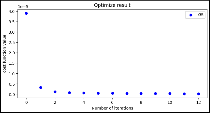
error_mass_gs = result_gs.cost_func_evolution
Solving direct problem with founded phase profile
[194]:
layer = elements.DiffractiveLayer(
simulation_parameters=sim_params,
mask=phase_distribution_gs
)
field_after_layer = layer.forward(incident_wavefront=incident_wavefront)
output_field_retrieved = free_space.forward(incident_wavefront=field_after_layer)
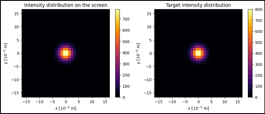
target_intensity_retrieved = output_field_retrieved.intensity
[195]:
fig, ax = plt.subplots(
    1, 2, figsize=(11, 4), edgecolor='black', linewidth=3, frameon=True
)

scale_factor = 1e5
x_grid_scaled = x_grid * scale_factor
y_grid_scaled = y_grid * scale_factor

im1 = ax[0].pcolormesh(x_grid_scaled, y_grid_scaled, target_intensity_retrieved, cmap='inferno')
ax[0].set_aspect('equal')
ax[0].set_title(r'Intensity distribution on the screen')
ax[0].set_xlabel('$x$ [$10^{-5}$ m]')
ax[0].set_ylabel('$y$ [$10^{-5}$ m]')
ax[0].set_xlim(-w0 / 6 * scale_factor, w0 / 6 * scale_factor)
ax[0].set_ylim(-w0 / 6 * scale_factor, w0 / 6 * scale_factor)
fig.colorbar(im1, ax=ax[0])

im2 = ax[1].pcolormesh(x_grid_scaled, y_grid_scaled, target_intensity, cmap='inferno')
ax[1].set_aspect('equal')
ax[1].set_title('Target intensity distribution')
ax[1].set_xlabel('$x$ [$10^{-5}$ m]')
ax[1].set_ylabel('$y$ [$10^{-5}$ m]')
ax[1].set_xlim(-w0 / 6 * scale_factor, w0 / 6 * scale_factor)
ax[1].set_ylim(-w0 / 6 * scale_factor, w0 / 6 * scale_factor)
fig.colorbar(im2, ax=ax[1])

plt.show()
[196]:
fig, ax = plt.subplots(
1, 2, figsize=(11, 4), edgecolor='black', linewidth=3, frameon=True
)
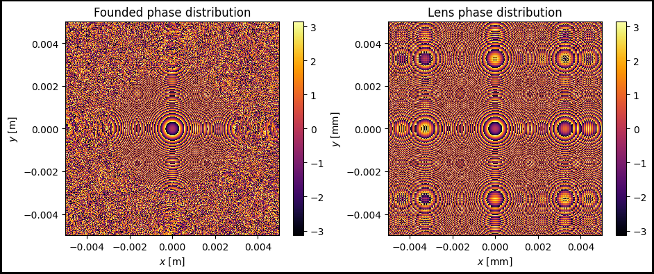
im1 = ax[0].pcolormesh(x_grid, y_grid, phase_distribution_gs, cmap='inferno')
ax[0].set_aspect('equal')
ax[0].set_title('Founded phase distribution')
ax[0].set_xlabel('$x$ [m]')
ax[0].set_ylabel('$y$ [m]')
fig.colorbar(im1)
im2 = ax[1].pcolormesh(x_grid, y_grid, torch.real(torch.log(lens.transmission_function) / 1j), cmap='inferno')
ax[1].set_aspect('equal')
ax[1].set_title('Lens phase distribution')
ax[1].set_xlabel('$x$ [mm]')
ax[1].set_ylabel('$y$ [mm]')
fig.colorbar(im2)
[196]:
<matplotlib.colorbar.Colorbar at 0x2689c55bb50>
[197]:
fig, ax = plt.subplots(figsize=(8.5, 4), edgecolor='black', linewidth=3, frameon=True
)

ax.set_title(r'Optimize result')
ax.set_xlabel('Number of iterations')
ax.set_ylabel('cost function value')

n_gs = np.arange(0, niter_gs+1)
ax.scatter(n_gs, error_mass_gs, label='GS', color='blue')

ax.legend()
[197]:
<matplotlib.legend.Legend at 0x2689c5db950>