Feed-forward Diffractive Optical Neural Network for MNIST task
In that example notebook we will make some experiments^ based on a n opticel network architecture proposed in the article.
Imports
[1]:
import os
import sys
import random
[2]:
import time
[3]:
import numpy as np
[4]:
import torch
from torch.utils.data import Dataset
[5]:
from torch import nn
[6]:
import torchvision
import torchvision.transforms as transforms
[7]:
from torchvision.transforms import InterpolationMode
[8]:
# our library
from svetlanna import SimulationParameters
from svetlanna.parameters import BoundedParameter
[9]:
# our library
from svetlanna import Wavefront
from svetlanna import elements
from svetlanna.setup import LinearOpticalSetup
from svetlanna.detector import Detector, DetectorProcessorClf
[10]:
from svetlanna.transforms import ToWavefront
[11]:
# datasets of wavefronts
from src.wf_datasets import DatasetOfWavefronts
from src.wf_datasets import IlluminatedApertureDataset
[12]:
from tqdm import tqdm
[13]:
import json
[14]:
from datetime import datetime
[15]:
import matplotlib.pyplot as plt
import matplotlib.patches as patches
from matplotlib.path import Path

plt.style.use('dark_background')
%matplotlib inline
# %config InlineBackend.figure_format = 'retina'
0. Experiment parameters
[16]:
working_frequency = 0.4 * 1e12 # [Hz]
C_CONST = 299_792_458  # [m / s]
[17]:
EXP_NUMBER = 1
[18]:
EXP_CONDITIONS = {
    # SIMULATION PARAMS
    'wavelength'  : C_CONST / working_frequency,  # [m]
    'layer_size_m': 8 * 1e-2 / 2 * 3,  # [m] - x and y sizes are equal!
    'layer_nodes' : int(100 / 2 * 3),  # 100,
    # TOOLS
    'tensorboard' : True,  # to use tensorboard or not!
    # DATASET
    'digit_resize' : 17,  # the actual digit size after resize (in nodes)
    'ds_apertures': True,  # if dataset is created with diigit-shaped apertures (True) or with direct modulation (False)
        # must be specified if 'ds_apertures' == False, values: 'amp', 'phase' or 'both'
    'ds_modulation': None,
        # must be specified if 'ds_apertures' == True
    'gauss_waist_radius': 2e-2,  # [m] - gaussian beam for dataset creation
    'distance_to_aperture': 3e-2,  # [m]
    # SETUP
    'propagator': 'AS',  # FreeSpase propagation method: 'AS' or 'fresnel' (also needed for dataset with apertures)
        # diffractive layers
    'n_diff_layers': 5,  # number of diffractive layers
    'diff_layer_max_phase': torch.pi,  # maximal phase for each DiffractiveLayer
    'diff_layer_mask_init': 'const',  # initialization of DiffractiveLayer masks: 'const' or 'random'
    'diff_layers_seeds': 123,  # if 'random': seed to generate seeds to init all masks!
        # free space
    'layers_distance': 3e-2,  # [m], distance between layers
        # apertures
    'add_apertures': True,  # if True - adds square apertures (in the middle) before each diffractive layer
    'apertures_size': (50, 50),  # size of additional apertures in a setup
        # detector
    'detector_zones': 'segments',  # form of a detector zones: 'squares' or 'circles' or 'strips'
    'detector_transpose': False,  # transpose detector or not (makes 'strips' horizontal instead of vertical)
    # TRAINING PROCESS
    'train_bs': 8,
    'val_bs': 20,  # batch sizes
    'train_split_seed': 178,  # seed for a data split on train/validation
    'epochs': 10,
}
[19]:
# import SummaryWriter from tensorboard

if 'tensorboard' in EXP_CONDITIONS.keys():
    if EXP_CONDITIONS['tensorboard']:

        from torch.utils.tensorboard import SummaryWriter
[20]:
today_date = datetime.today().strftime('%d-%m-%Y')

RESULTS_FOLDER = (
    f'models/03_mnist_experiments/{today_date}_experiment_{EXP_NUMBER:02d}'
)

RESULTS_FOLDER
[20]:
'models/03_mnist_experiments/13-12-2024_experiment_01'
[21]:
if not os.path.exists(RESULTS_FOLDER):
    os.makedirs(RESULTS_FOLDER)
[22]:
# save experiment conditions
json.dump(EXP_CONDITIONS, open(f'{RESULTS_FOLDER}/conditions.json', 'w'))
[23]:
# OR read conditions from file:
# EXP_CONDITIONS = json.load(open(f'{RESULTS_FOLDER}/conditions.json))
# print(EXP_CONDITIONS)
[ ]:
1. Simulation parameters
[24]:
working_wavelength = EXP_CONDITIONS['wavelength']  # [m]
print(f'lambda = {working_wavelength * 1e6:.3f} um')
lambda = 749.481 um
[25]:
# physical size of each layer (from the article) - (8 x 8) [cm]
x_layer_size_m = EXP_CONDITIONS['layer_size_m']  # [m]
y_layer_size_m = x_layer_size_m
[26]:
# number of neurons in simulation
x_layer_nodes = EXP_CONDITIONS['layer_nodes']
y_layer_nodes = x_layer_nodes
[27]:
print(f'Layer size (neurons): {x_layer_nodes} x {y_layer_nodes} = {x_layer_nodes * y_layer_nodes}')
Layer size (neurons): 150 x 150 = 22500
[28]:
neuron_size = x_layer_size_m / x_layer_nodes  # [m]  increase two times!
print(f'Neuron size = {neuron_size * 1e6:.3f} um')
Neuron size = 800.000 um
[29]:
# simulation parameters for the rest of the notebook

SIM_PARAMS = SimulationParameters(
    axes={
        'W': torch.linspace(-x_layer_size_m / 2, x_layer_size_m / 2, x_layer_nodes),
        'H': torch.linspace(-y_layer_size_m / 2, y_layer_size_m / 2, y_layer_nodes),
        'wavelength': working_wavelength,  # only one wavelength!
    }
)
[ ]:
2. Dataset preparation (Data Engineer)
2.1. MNIST Dataset
[30]:
# initialize a directory for a dataset
MNIST_DATA_FOLDER = './data'  # folder to store data
2.1.1. Train/Test datasets of images
[31]:
# TRAIN (images)
mnist_train_ds = torchvision.datasets.MNIST(
    root=MNIST_DATA_FOLDER,
    train=True,  # for train dataset
    download=False,
)
[32]:
# TEST (images)
mnist_test_ds = torchvision.datasets.MNIST(
    root=MNIST_DATA_FOLDER,
    train=False,  # for test dataset
    download=False,
)
[33]:
print(f'Train data: {len(mnist_train_ds)}')
print(f'Test data : {len(mnist_test_ds)}')
Train data: 60000
Test data : 10000
2.1.2. Train/Test datasets of wavefronts
[34]:
DS_WITH_APERTURES = EXP_CONDITIONS['ds_apertures']
# if True we use IlluminatedApertureDataset to create datasets of Wavefronts
# else - DatasetOfWavefronts
DS_WITH_APERTURES
[34]:
True
[35]:
# select modulation type for DatasetOfWavefronts if DS_WITH_APERTURES == False
MODULATION_TYPE = EXP_CONDITIONS['ds_modulation']  # 'phase', 'amp', 'amp&phase'

# select method and distance for a FreeSpace in IlluminatedApertureDataset
DS_METHOD = EXP_CONDITIONS['propagator']
DS_DISTANCE = EXP_CONDITIONS['distance_to_aperture']  # [m]

DS_BEAM = Wavefront.gaussian_beam(
    simulation_parameters=SIM_PARAMS,
    waist_radius=EXP_CONDITIONS['gauss_waist_radius'],  # [m]
)
[ ]:
[36]:
# image resize to match SimulationParameters
resize_y = EXP_CONDITIONS['digit_resize']
resize_x = resize_y  # shape for transforms.Resize

pad_top = int((y_layer_nodes - resize_y) / 2)
pad_bottom = y_layer_nodes - pad_top - resize_y
pad_left = int((x_layer_nodes - resize_x) / 2)
pad_right = x_layer_nodes - pad_left - resize_x  # params for transforms.Pad
[37]:
# compose all transforms for DatasetOfWavefronts
image_transform_for_ds = transforms.Compose(
  [
      transforms.ToTensor(),
      transforms.Resize(
          size=(resize_y, resize_x),
          interpolation=InterpolationMode.NEAREST,
      ),
      transforms.Pad(
          padding=(
              pad_left,  # left padding
              pad_top,  # top padding
              pad_right,  # right padding
              pad_bottom  # bottom padding
          ),
          fill=0,
      ),  # padding to match sizes!
      ToWavefront(modulation_type=MODULATION_TYPE)  # <- select modulation type!!!
  ]
)

# compose all transforms for IlluminatedApertureDataset
image_to_aperture = transforms.Compose(
  [
      transforms.ToTensor(),
      transforms.Resize(
          size=(resize_y, resize_x),
          interpolation=InterpolationMode.NEAREST,
      ),
      transforms.Pad(
          padding=(
              pad_left,  # left padding
              pad_top,  # top padding
              pad_right,  # right padding
              pad_bottom  # bottom padding
          ),
          fill=0,
      ),  # padding to match sizes!
  ]
)
[38]:
# TRAIN dataset of WAVEFRONTS
if not DS_WITH_APERTURES:
    mnist_wf_train_ds = DatasetOfWavefronts(
        init_ds=mnist_train_ds,  # dataset of images
        transformations=image_transform_for_ds,  # image transformation
        sim_params=SIM_PARAMS,  # simulation parameters
    )
else:
    mnist_wf_train_ds = IlluminatedApertureDataset(
        init_ds=mnist_train_ds,  # dataset of images
        transformations=image_to_aperture,  # image transformation
        sim_params=SIM_PARAMS,  # simulation parameters
        beam_field=DS_BEAM,
        distance=DS_DISTANCE,
        method=DS_METHOD,
    )
[39]:
# TEST dataset of WAVEFRONTS
if not DS_WITH_APERTURES:
    mnist_wf_test_ds = DatasetOfWavefronts(
        init_ds=mnist_test_ds,  # dataset of images
        transformations=image_transform_for_ds,  # image transformation
        sim_params=SIM_PARAMS,  # simulation parameters
    )
else:
    mnist_wf_test_ds = IlluminatedApertureDataset(
        init_ds=mnist_test_ds,  # dataset of images
        transformations=image_to_aperture,  # image transformation
        sim_params=SIM_PARAMS,  # simulation parameters
        beam_field=DS_BEAM,
        distance=DS_DISTANCE,
        method=DS_METHOD,
    )
[40]:
print(f'Train data: {len(mnist_wf_train_ds)}')
print(f'Test data : {len(mnist_wf_test_ds)}')
Train data: 60000
Test data : 10000
[41]:
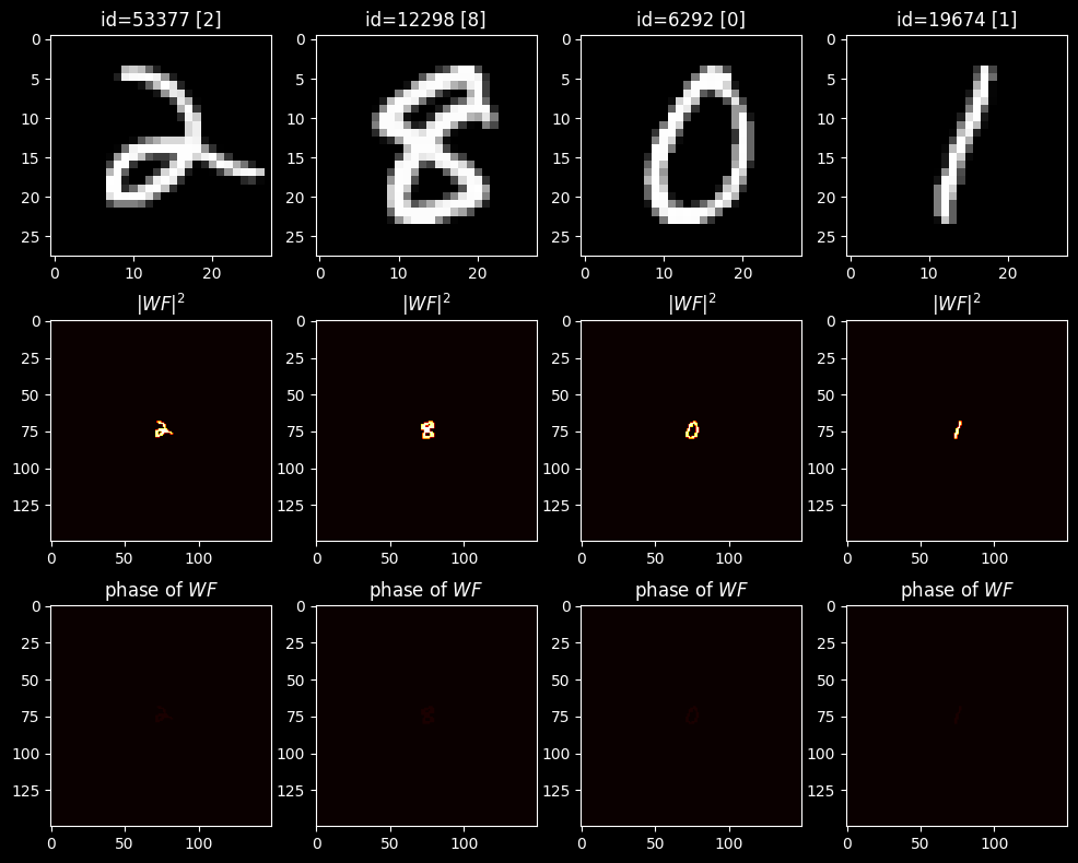
# plot several EXAMPLES from TRAIN dataset
n_examples= 4  # number of examples to plot
# choosing indecies of images (from train) to plot
random.seed(78)
train_examples_ids = random.sample(range(len(mnist_train_ds)), n_examples)

all_examples_wavefronts = []
cmap = 'hot'

n_lines = 3
fig, axs = plt.subplots(n_lines, n_examples, figsize=(n_examples * 3, n_lines * 3.2))
for ind_ex, ind_train in enumerate(train_examples_ids):
    image, label = mnist_train_ds[ind_train]

    axs[0][ind_ex].set_title(f'id={ind_train} [{label}]')
    axs[0][ind_ex].imshow(image, cmap='gray')

    wavefront, wf_label = mnist_wf_train_ds[ind_train]
    assert isinstance(wavefront, Wavefront)

    all_examples_wavefronts.append(wavefront)

    axs[1][ind_ex].set_title(f'$|WF|^2$')
    # here we can plot intensity for a wavefront
    axs[1][ind_ex].imshow(
        wavefront.intensity[0], cmap=cmap,
        vmin=0, vmax=1
    )

    axs[2][ind_ex].set_title(f'phase of $WF$')
    axs[2][ind_ex].imshow(
        wavefront.phase[0], cmap=cmap,
        vmin=0, vmax= 2 * torch.pi
    )

plt.show()
[ ]:
3. Optical network
[42]:
NUM_OF_DIFF_LAYERS = EXP_CONDITIONS['n_diff_layers']  # number of diffractive layers
FREE_SPACE_DISTANCE = EXP_CONDITIONS['layers_distance']  # [m]
3.1. Architecture
3.1.1. List of Elements
To help with the 3D-printing and fabrication of the \(D^2NN\) design, a sigmoid function was used to limit the phase value of each neuron to \(0-2π\) and \(0-π\), for imaging and classifier networks, respectively.
[43]:
MAX_PHASE = EXP_CONDITIONS['diff_layer_max_phase']
[44]:
from src.for_setup import get_const_free_space, get_random_diffractive_layer
from torch.nn import functional
Function to construct a list of elements:
[45]:
# WE WILL ADD APERTURES BEFORE EACH DIFFRACTIVE LAYER OF THE SIZE:
ADD_APERTURES = EXP_CONDITIONS['add_apertures']
APERTURE_SZ = EXP_CONDITIONS['apertures_size']
[46]:
def get_elements_list(
    num_layers,
    simulation_parameters: SimulationParameters,
    freespace_method,
    masks_seeds,
    apertures=False,
    aperture_size=(100, 100)
):
    """
    Composes a list of elements for setup.
        Optical system: FS|DL|FS|...|FS|DL|FS|Detector
    ...

    Parameters
    ----------
    num_layers : int
        Number of layers in the system.
    simulation_parameters : SimulationParameters()
        A simulation parameters for a task.
    freespace_method : str
        Propagation method for free spaces in a setup.
    masks_seeds : torch.Tensor()
        Torch tensor of random seeds to generate masks for diffractive layers.

    Returns
    -------
    elements_list : list(Element)
        List of Elements for an optical setup.
    """
    elements_list = []  # list of elements

    if apertures:  # equal masks for all apertures (select a part in the middle)
        aperture_mask = torch.ones(size=aperture_size)

        y_nodes, x_nodes = simulation_parameters.axes_size(axs=('H', 'W'))
        y_mask, x_mask = aperture_mask.size()
        pad_top = int((y_nodes - y_mask) / 2)
        pad_bottom = y_nodes - pad_top - y_mask
        pad_left = int((x_nodes - x_mask) / 2)
        pad_right = x_nodes - pad_left - x_mask  # params for transforms.Pad

        # padding transform to match aperture size with simulation parameters
        aperture_mask = functional.pad(
            input=aperture_mask,
            pad=(pad_left, pad_right, pad_top, pad_bottom),
            mode='constant',
            value=0
        )

    # compose architecture
    for ind_layer in range(num_layers):
        if ind_layer == 0:
            # first FreeSpace layer before first DiffractiveLayer
            elements_list.append(
                get_const_free_space(
                    simulation_parameters,  # simulation parameters for the notebook
                    FREE_SPACE_DISTANCE,  # in [m]
                    freespace_method=freespace_method,
                )
            )

        # add aperture before each diffractive layer
        if apertures:
            elements_list.append(
                elements.Aperture(
                    simulation_parameters=simulation_parameters,
                    mask=nn.Parameter(aperture_mask, requires_grad=False)
                )
            )

        # add DiffractiveLayer
        elements_list.append(
            get_random_diffractive_layer(
                simulation_parameters,  # simulation parameters for the notebook
                mask_seed=masks_seeds[ind_layer].item(),
                max_phase=MAX_PHASE
            )
        )
        # add FreeSpace
        elements_list.append(
            get_const_free_space(
                simulation_parameters,  # simulation parameters for the notebook
                FREE_SPACE_DISTANCE,  # in [m]
                freespace_method=freespace_method,
            )
        )

    # add Detector in the end of the system!
    elements_list.append(
        Detector(
            simulation_parameters=simulation_parameters,
            func='intensity'  # detector that returns intensity
        )
    )

    return elements_list
Constants for a setup initialization:
[47]:
FREESPACE_METHOD = EXP_CONDITIONS['propagator'] # TODO: 'AS' returns nan's?

if EXP_CONDITIONS['diff_layer_mask_init'] == 'random':
    MASKS_SEEDS = torch.randint(
        low=0, high=100,
        size=(NUM_OF_DIFF_LAYERS,),
        generator=torch.Generator().manual_seed(EXP_CONDITIONS['diff_layers_seeds'])
        # to generate the same set of initial masks
    )  # for the same random generation

if EXP_CONDITIONS['diff_layer_mask_init'] == 'const':
    MASKS_SEEDS = torch.ones(size=(NUM_OF_DIFF_LAYERS,)) * torch.pi / 2  # constant masks init

MASKS_SEEDS
[47]:
tensor([1.5708, 1.5708, 1.5708, 1.5708, 1.5708])
[ ]:
3.1.2. Compose LinearOpticalSetup
[48]:
def get_setup(
    simulation_parameters,
    num_layers,
    apertures=False,
    aperture_size=(100,100)
):
    """
    Returns an optical setup. Recreates all elements.
    """
    elements_list = get_elements_list(
        num_layers,
        simulation_parameters,
        FREESPACE_METHOD,
        MASKS_SEEDS,
        apertures=apertures,
        aperture_size=aperture_size
    )  # recreate a list of elements

    return LinearOpticalSetup(elements=elements_list)
[49]:
lin_optical_setup = get_setup(
    SIM_PARAMS,
    NUM_OF_DIFF_LAYERS,
    apertures=ADD_APERTURES,
    aperture_size=APERTURE_SZ
)
# Comment: Lin - a surname of the first author of the article
[50]:
lin_optical_setup.net
[50]:
Sequential(
  (0): FreeSpace()
  (1): Aperture()
  (2): DiffractiveLayer()
  (3): FreeSpace()
  (4): Aperture()
  (5): DiffractiveLayer()
  (6): FreeSpace()
  (7): Aperture()
  (8): DiffractiveLayer()
  (9): FreeSpace()
  (10): Aperture()
  (11): DiffractiveLayer()
  (12): FreeSpace()
  (13): Aperture()
  (14): DiffractiveLayer()
  (15): FreeSpace()
  (16): Detector()
)
[ ]:
[51]:
example_wf = mnist_wf_train_ds[128][0]
[52]:
mnist_wf_train_ds[128][1]
[52]:
1
[53]:
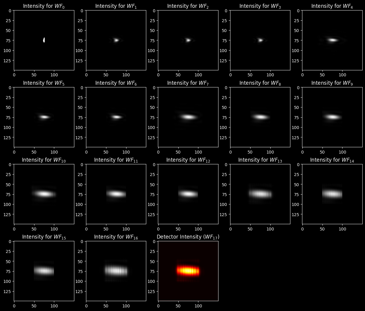
setup_scheme, wavefronts = lin_optical_setup.stepwise_forward(example_wf)
[54]:
print(setup_scheme)  # prints propagation scheme

n_cols = 5  # number of columns to plot all wavefronts during propagation
n_rows = (len(lin_optical_setup.net) // n_cols) + 1

to_plot = 'amp'  # <--- chose what to plot
cmap = 'grey'  # choose colormaps
detector_cmap = 'hot'

# create a figure with subplots
fig, axs = plt.subplots(n_rows, n_cols, figsize=(n_cols * 3, n_rows * 3.2))

# turn off unecessary axes
for ind_row in range(n_rows):
    for ind_col in range(n_cols):
        ax_this = axs[ind_row][ind_col]
        if ind_row * n_cols + ind_col >= len(wavefronts):
            ax_this.axis('off')

# plot wavefronts
for ind_wf, wavefront in enumerate(wavefronts):
    ax_this = axs[ind_wf // n_cols][ind_wf % n_cols]

    if to_plot == 'phase':
        # plot angle for each wavefront, because intensities pictures are indistinguishable from each other
        if ind_wf < len(wavefronts) - 1:
            ax_this.set_title('Phase for $WF_{' + f'{ind_wf}' + '}$')
            ax_this.imshow(
                wavefront[0].phase.detach().numpy(), cmap=cmap,
                vmin=0, vmax=2 * torch.pi
            )
        else:  # (not a wavefront!)
            ax_this.set_title('Detector phase ($WF_{' + f'{ind_wf}' + '})$')
            # Detector has no phase!

    if to_plot == 'amp':
        # plot angle for each wavefront, because intensities pictures are indistinguishable from each other
        if ind_wf < len(wavefronts) - 1:
            ax_this.set_title('Intensity for $WF_{' + f'{ind_wf}' + '}$')
            ax_this.imshow(
                wavefront[0].intensity.detach().numpy(), cmap=cmap,
                # vmin=0, vmax=max_intensity  # uncomment to make the same limits
            )
        else:  # Detector output (not a wavefront!)
            ax_this.set_title('Detector Intensity ($WF_{' + f'{ind_wf}' + '})$')
            ax_this.imshow(
                wavefront[0].detach().numpy(), cmap=detector_cmap,
                # vmin=0, vmax=max_intensity  # uncomment to make the same limits
            )

    # Comment: Detector output is Tensor! It has no methods of Wavefront (like .phase or .intensity)!

plt.show()
-(0)-> [1. FreeSpace] -(1)-> [2. Aperture] -(2)-> [3. DiffractiveLayer] -(3)-> [4. FreeSpace] -(4)-> [5. Aperture] -(5)-> [6. DiffractiveLayer] -(6)-> [7. FreeSpace] -(7)-> [8. Aperture] -(8)-> [9. DiffractiveLayer] -(9)-> [10. FreeSpace] -(10)-> [11. Aperture] -(11)-> [12. DiffractiveLayer] -(12)-> [13. FreeSpace] -(13)-> [14. Aperture] -(14)-> [15. DiffractiveLayer] -(15)-> [16. FreeSpace] -(16)-> [17. Detector] -(17)->
[ ]:
3.1.3 Detector processor
[55]:
number_of_classes = 10
[56]:
import src.detector_segmentation as detector_segmentation
# Functions to segment detector: squares_mnist, circles, angular_segments
[57]:
if ADD_APERTURES or APERTURE_SZ:
    y_detector_nodes, x_detector_nodes = APERTURE_SZ
else:
    y_detector_nodes, x_detector_nodes = SIM_PARAMS.axes_size(axs=('H', 'W'))
[58]:
ADD_APERTURES
[58]:
True
[ ]:
[59]:
detector_squares_mask = detector_segmentation.squares_mnist(
    y_detector_nodes, x_detector_nodes,  # size of a detector or an aperture (in the middle of detector)
    SIM_PARAMS
)
[60]:
detector_circles_mask = detector_segmentation.circles(
    y_detector_nodes, x_detector_nodes,  # size of a detector or an aperture (in the middle of detector)
    number_of_classes,
    SIM_PARAMS
)
[61]:
detector_angles_mask = detector_segmentation.angular_segments(
    y_detector_nodes, x_detector_nodes,  # size of a detector or an aperture (in the middle of detector)
    number_of_classes,
    SIM_PARAMS
)
[ ]:
[62]:
CIRCLES_ZONES = EXP_CONDITIONS['detector_zones'] == 'circles'
CIRCLES_ZONES
[62]:
False
[63]:
if EXP_CONDITIONS['detector_zones'] == 'circles':
selected_mask = detector_circles_mask
print('circles selected!')
if EXP_CONDITIONS['detector_zones'] == 'squares':
selected_mask = detector_squares_mask
print('squares selected!')
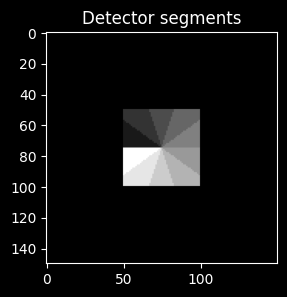
if EXP_CONDITIONS['detector_zones'] == 'segments':
selected_mask = detector_angles_mask
print('angular segments selected!')
if EXP_CONDITIONS['detector_zones'] == 'strips':
selected_mask = None
print('strips selected!')
angular segments selected!
[64]:
detector_processor = DetectorProcessorClf(
    num_classes=number_of_classes,
    simulation_parameters=SIM_PARAMS,
    segmented_detector=selected_mask,  # choose a mask!
    segments_zone_size=APERTURE_SZ
)
[65]:
if 'detector_transpose' in EXP_CONDITIONS.keys():
    if EXP_CONDITIONS['detector_transpose']:
        detector_processor.segmented_detector = detector_processor.segmented_detector.T
[66]:
fig, ax0 = plt.subplots(1, 1, figsize=(3, 3))

ax0.set_title(f'Detector segments')
ax0.imshow(detector_processor.segmented_detector, cmap='grey')

plt.show()
[ ]:
[67]:
ZONES_HIGHLIGHT_COLOR = 'w'
ZONES_LW = 0.5
selected_detector_mask = detector_processor.segmented_detector.clone().detach()
[68]:
def get_zones_patches(detector_mask):
    """
    Returns a list of patches to draw zones in final visualisation
    """
    zones_patches = []

    if EXP_CONDITIONS['detector_zones'] == 'circles':
        for ind_class in range(number_of_classes):
            # use `circles_radiuses`, `x_layer_size_m`, `x_layer_nodes`
            rad_this = (circles_radiuses[ind_class] / x_layer_size_m * x_layer_nodes)

            zone_circ = patches.Circle(
                (x_layer_nodes / 2, y_layer_nodes / 2),
                rad_this,
                linewidth=ZONES_LW,
                edgecolor=ZONES_HIGHLIGHT_COLOR,
                facecolor='none'
            )

            zones_patches.append(zone_circ)
    else:
        if EXP_CONDITIONS['detector_zones'] == 'segments':
            class_segment_angle = 2 * torch.pi / number_of_classes
            len_lines_nodes = int(x_layer_nodes / 2)

            delta = 0.5
            idx_y, idx_x = (detector_mask > -1).nonzero(as_tuple=True)
            zone_rect = patches.Rectangle(
                (idx_x[0] - delta, idx_y[0] - delta),
                idx_x[-1] - idx_x[0] + 2 * delta, idx_y[-1] - idx_y[0] + 2 * delta,
                linewidth=ZONES_LW,
                edgecolor=ZONES_HIGHLIGHT_COLOR,
                facecolor='none'
            )
            zones_patches.append(zone_rect)

            ang = torch.pi
            x_center, y_center = int(x_layer_nodes / 2), int(y_layer_nodes / 2)
            for ind_class in range(number_of_classes):
                path_line = Path(
                    [
                        (x_center, y_center),
                        (
                            x_center + len_lines_nodes * np.cos(ang),
                            y_center + len_lines_nodes * np.sin(ang)
                        ),
                    ],
                    [
                        Path.MOVETO,
                        Path.LINETO
                    ]
                )
                bound_line = patches.PathPatch(
                    path_line,
                    facecolor='none',
                    lw=ZONES_LW,
                    edgecolor=ZONES_HIGHLIGHT_COLOR,
                )

                zones_patches.append(bound_line)

                ang += class_segment_angle
        else:
            delta = 0.5

            for ind_class in range(number_of_classes):
                idx_y, idx_x = (detector_mask == ind_class).nonzero(as_tuple=True)

                zone_rect = patches.Rectangle(
                    (idx_x[0] - delta, idx_y[0] - delta),
                    idx_x[-1] - idx_x[0] + 2 * delta, idx_y[-1] - idx_y[0] + 2 * delta,
                    linewidth=ZONES_LW,
                    edgecolor=ZONES_HIGHLIGHT_COLOR,
                    facecolor='none'
                )

                zones_patches.append(zone_rect)

    return zones_patches
[ ]:
4. Training of the network
Variables at the moment
lin_optical_setup:LinearOpticalSetup– a linear optical network composed of Elementsdetector_processor:DetectorProcessorClf– this layer process an image from the detector and calculates probabilities of belonging to classes.
[69]:
DEVICE = torch.device('cuda' if torch.cuda.is_available() else 'cpu')

# if DEVICE == torch.device('cpu'):
#     DEVICE = torch.device('mps' if torch.backends.mps.is_available() else 'cpu')

DEVICE
[69]:
device(type='cpu')
4.1. Prepare some stuff for training
4.1.1. DataLoader’s
[70]:
train_bs = EXP_CONDITIONS['train_bs']  # a batch size for training set
val_bs = EXP_CONDITIONS['val_bs']
Forthis task, phase-only transmission masks weredesigned by training a five-layer \(D^2 NN\) with \(55000\) images (\(5000\) validation images) from theMNIST (Modified National Institute of Stan-dards and Technology) handwritten digit data-base.
[71]:
# mnist_wf_train_ds
train_wf_ds, val_wf_ds = torch.utils.data.random_split(
    dataset=mnist_wf_train_ds,
    lengths=[55000, 5000],  # sizes from the article
    generator=torch.Generator().manual_seed(EXP_CONDITIONS['train_split_seed'])  # for reproducibility
)
[72]:
train_wf_loader = torch.utils.data.DataLoader(
    train_wf_ds,
    batch_size=train_bs,
    shuffle=True,
    # num_workers=2,
    drop_last=False,
)

val_wf_loader = torch.utils.data.DataLoader(
    val_wf_ds,
    batch_size=val_bs,
    shuffle=False,
    # num_workers=2,
    drop_last=False,
)
[ ]:
4.1.2. Optimizer and loss function
Info from a supplementary material for MNIST classification:
We used the stochastic gradient descent algorithm, Adam, to back-propagate the errors and update the layers of the network to minimize the loss function.
[73]:
optimizer_clf = torch.optim.Adam(
    params=lin_optical_setup.net.parameters()  # NETWORK PARAMETERS!
)
[74]:
loss_func_clf = nn.CrossEntropyLoss()
loss_func_name = 'CE loss'
[ ]:
4.1.3. Training and evaluation loops
[75]:
from src.clf_loops import onn_train_clf, onn_validate_clf
[ ]:
4.2. Training of the optical network
4.2.1. Before training
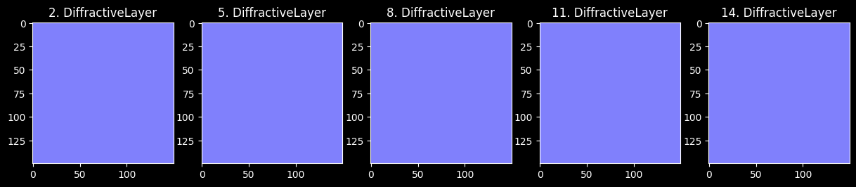
[91]:
n_cols = NUM_OF_DIFF_LAYERS  # number of columns for DiffractiveLayer's masks visualization
n_rows = 1

lin_architecture_elements_list = get_elements_list(
    NUM_OF_DIFF_LAYERS,
    SIM_PARAMS,
    FREESPACE_METHOD,
    MASKS_SEEDS,
    apertures=ADD_APERTURES,
    aperture_size=APERTURE_SZ
)

cmap = 'gist_stern'

# plot wavefronts phase
fig, axs = plt.subplots(n_rows, n_cols, figsize=(n_cols * 3, n_rows * 3.2))
ind_diff_layer = 0

for ind_layer, layer in enumerate(lin_architecture_elements_list):
    if isinstance(layer, elements.DiffractiveLayer):  # plot masks for Diffractive layers
        if n_rows > 1:
            ax_this = axs[ind_diff_layer // n_cols][ind_diff_layer % n_cols]
        else:
            ax_this = axs[ind_diff_layer % n_cols]

        ax_this.set_title(f'{ind_layer}. DiffractiveLayer')

        im = ax_this.imshow(
            layer.mask.detach().numpy(), cmap=cmap,
            vmin=0, vmax=MAX_PHASE
        )

        ind_diff_layer += 1

plt.show()
[ ]:
[ ]:
[77]:
lin_optical_setup = get_setup(
    SIM_PARAMS.to(DEVICE),
    NUM_OF_DIFF_LAYERS,
    apertures=ADD_APERTURES,
    aperture_size=APERTURE_SZ
)
[78]:
lin_optical_setup.net = lin_optical_setup.net.to(DEVICE)

SIM_PARAMS = SIM_PARAMS.to(DEVICE)  # IMPORTANT!
detector_processor = detector_processor.to(DEVICE)
[ ]:
[79]:
test_wf_loader = torch.utils.data.DataLoader(
    mnist_wf_test_ds,
    batch_size=10,
    shuffle=False,
    # num_workers=2,
    drop_last=False,
)  # data loader for a test MNIST data
[80]:
test_losses_0, _, test_accuracy_0 = onn_validate_clf(
    lin_optical_setup.net,  # optical network composed in 3.
    test_wf_loader,  # dataloader of training set
    detector_processor,  # detector processor
    loss_func_clf,
    device=DEVICE,
    show_process=True,
)  # evaluate the model

print(
    'Results before training on TEST set:\n' +
    f'\t{loss_func_name} : {np.mean(test_losses_0):.6f}\n' +
    f'\tAccuracy : {(test_accuracy_0*100):>0.1f} %'
)
validation: 100%|████████████████████████████████████████████████████████████████████████| 1000/1000 [00:19<00:00, 50.14it/s]
Results before training on TEST set:
        CE loss : 2.304648
        Accuracy : 9.7 %
[ ]:
4.2.2. Training
[111]:
n_epochs = EXP_CONDITIONS['epochs']
print_each = 1  # print each n'th epoch info
[112]:
scheduler = None # sheduler for a lr tuning during training
[113]:
# Recreate a system to restart training!

lin_optical_setup = get_setup(
    SIM_PARAMS.to(DEVICE),
    NUM_OF_DIFF_LAYERS,
    apertures=ADD_APERTURES,
    aperture_size=APERTURE_SZ
)

# Linc optimizer to a recreated net!
optimizer_clf = torch.optim.Adam(
    params=lin_optical_setup.net.parameters()  # NETWORK PARAMETERS!
)
[114]:
lin_optical_setup.net
[114]:
Sequential(
  (0): FreeSpace()
  (1): Aperture()
  (2): DiffractiveLayer()
  (3): FreeSpace()
  (4): Aperture()
  (5): DiffractiveLayer()
  (6): FreeSpace()
  (7): Aperture()
  (8): DiffractiveLayer()
  (9): FreeSpace()
  (10): Aperture()
  (11): DiffractiveLayer()
  (12): FreeSpace()
  (13): Aperture()
  (14): DiffractiveLayer()
  (15): FreeSpace()
  (16): Detector()
)
[115]:
lin_optical_setup.net = lin_optical_setup.net.to(DEVICE)

SIM_PARAMS = SIM_PARAMS.to(DEVICE)  # IMPORTANT!
detector_processor = detector_processor.to(DEVICE)  # detector processor also must be on device!
[116]:
# tensorboard writer
if EXP_CONDITIONS['tensorboard']:
    # TODO: A custom name for a run?
    tensorboard_writer = SummaryWriter()
    print('Tensorboard writer created!')
Tensorboard writer created!
[ ]:
[ ]:
[117]:
train_epochs_losses = []
val_epochs_losses = []  # to store losses of each epoch

train_epochs_acc = []
val_epochs_acc = []  # to store accuracies

torch.manual_seed(98)  # for reproducability?

for epoch in range(n_epochs):
    if (epoch == 0) or ((epoch + 1) % print_each == 0):
        print(f'Epoch #{epoch + 1}: ', end='')
        show_progress = True
    else:
        show_progress = False

    # TRAIN
    start_train_time = time.time()  # start time of the epoch (train)
    train_losses, _, train_accuracy = onn_train_clf(
        lin_optical_setup.net,  # optical network composed in 3.
        train_wf_loader,  # dataloader of training set
        detector_processor,  # detector processor
        loss_func_clf,
        optimizer_clf,
        device=DEVICE,
        show_process=show_progress,
    )  # train the model
    mean_train_loss = np.mean(train_losses)

    if (epoch == 0) or ((epoch + 1) % print_each == 0):  # train info
        print('Training results')
        print(f'\t{loss_func_name} : {mean_train_loss:.6f}')
        print(f'\tAccuracy : {(train_accuracy*100):>0.1f} %')
        print(f'\t------------   {time.time() - start_train_time:.2f} s')

    # VALIDATION
    start_val_time = time.time()  # start time of the epoch (validation)
    val_losses, _, val_accuracy = onn_validate_clf(
        lin_optical_setup.net,  # optical network composed in 3.
        val_wf_loader,  # dataloader of validation set
        detector_processor,  # detector processor
        loss_func_clf,
        device=DEVICE,
        show_process=show_progress,
    )  # evaluate the model
    mean_val_loss = np.mean(val_losses)

    if (epoch == 0) or ((epoch + 1) % print_each == 0):  # validation info
        print('Validation results')
        print(f'\t{loss_func_name} : {mean_val_loss:.6f}')
        print(f'\tAccuracy : {(val_accuracy*100):>0.1f} %')
        print(f'\t------------   {time.time() - start_val_time:.2f} s')

    if scheduler:
        scheduler.step(mean_val_loss)

    # ---------------------------------------------------- TENSORBOARD SECTION
    if EXP_CONDITIONS['tensorboard']:
        #exprimentation tracking section: tensorboard
        tensorboard_writer.add_scalars(
            main_tag="Loss",
            tag_scalar_dict={
                "train_loss": mean_train_loss,
                "val_loss": mean_val_loss,
                "train_accuracy": train_accuracy,
                "val_accuracy": val_accuracy,
            },
            global_step=epoch
        )

        # image of SLM at each epoch
        diff_layer_number = 1
        for layer in lin_optical_setup.net:
            # save masks for Diffractive layers after each epoch
            if isinstance(layer, elements.DiffractiveLayer):
                mask_np = layer.mask.detach().unsqueeze(0).numpy()

                # TODO: Figure to add?
                # fig_this, ax_this =  plt.subplots(1, 1, figsize=(5, 4))
                # im_this = ax_this.imshow(
                #     layer.mask.detach().numpy(), cmap=cmap,
                #     vmin=0, vmax=MAX_PHASE
                # )
                # cbar_this = fig.colorbar(im_this)
                # im_this.set_clim(0, MAX_PHASE)

                # WRITE
                tensorboard_writer.add_image(
                    f'DiffractiveLayer_{diff_layer_number}',
                    mask_np,
                    global_step=epoch
                )
                diff_layer_number += 1
        print(f'\t-> tensorboarded')
    # ---------------------------------------------------- TENSORBOARD SECTION

    # save losses
    train_epochs_losses.append(mean_train_loss)
    val_epochs_losses.append(mean_val_loss)
    # seve accuracies
    train_epochs_acc.append(train_accuracy)
    val_epochs_acc.append(val_accuracy)
Epoch #1:
train: 100%|█████████████████████████████████████████████████████████████████████████████| 6875/6875 [05:09<00:00, 22.18it/s]
Training results
        CE loss : 2.026149
        Accuracy : 69.7 %
        ------------   309.92 s
validation: 100%|██████████████████████████████████████████████████████████████████████████| 250/250 [00:16<00:00, 15.28it/s]
Validation results
        CE loss : 1.976295
        Accuracy : 76.0 %
        ------------   16.36 s
        -> tensorboarded
Epoch #2:
train: 100%|█████████████████████████████████████████████████████████████████████████████| 6875/6875 [05:25<00:00, 21.11it/s]
Training results
        CE loss : 1.954368
        Accuracy : 78.8 %
        ------------   325.61 s
validation: 100%|██████████████████████████████████████████████████████████████████████████| 250/250 [00:17<00:00, 14.38it/s]
Validation results
        CE loss : 1.944904
        Accuracy : 78.9 %
        ------------   17.38 s
        -> tensorboarded
Epoch #3:
train: 100%|█████████████████████████████████████████████████████████████████████████████| 6875/6875 [05:15<00:00, 21.78it/s]
Training results
        CE loss : 1.932177
        Accuracy : 80.4 %
        ------------   315.66 s
validation: 100%|██████████████████████████████████████████████████████████████████████████| 250/250 [00:18<00:00, 13.83it/s]
Validation results
        CE loss : 1.927474
        Accuracy : 80.7 %
        ------------   18.08 s
        -> tensorboarded
Epoch #4:
train: 100%|█████████████████████████████████████████████████████████████████████████████| 6875/6875 [06:05<00:00, 18.79it/s]
Training results
        CE loss : 1.919771
        Accuracy : 81.1 %
        ------------   365.97 s
validation: 100%|██████████████████████████████████████████████████████████████████████████| 250/250 [00:19<00:00, 12.67it/s]
Validation results
        CE loss : 1.918410
        Accuracy : 81.6 %
        ------------   19.74 s
        -> tensorboarded
Epoch #5:
train: 100%|█████████████████████████████████████████████████████████████████████████████| 6875/6875 [06:09<00:00, 18.63it/s]
Training results
        CE loss : 1.911985
        Accuracy : 81.5 %
        ------------   369.08 s
validation: 100%|██████████████████████████████████████████████████████████████████████████| 250/250 [00:21<00:00, 11.77it/s]
Validation results
        CE loss : 1.911945
        Accuracy : 81.1 %
        ------------   21.25 s
        -> tensorboarded
Epoch #6:
train: 100%|█████████████████████████████████████████████████████████████████████████████| 6875/6875 [06:21<00:00, 18.02it/s]
Training results
        CE loss : 1.906370
        Accuracy : 81.9 %
        ------------   381.45 s
validation: 100%|██████████████████████████████████████████████████████████████████████████| 250/250 [00:19<00:00, 12.72it/s]
Validation results
        CE loss : 1.906746
        Accuracy : 82.1 %
        ------------   19.66 s
        -> tensorboarded
Epoch #7:
train: 100%|█████████████████████████████████████████████████████████████████████████████| 6875/6875 [06:52<00:00, 16.68it/s]
Training results
        CE loss : 1.902148
        Accuracy : 82.1 %
        ------------   412.09 s
validation: 100%|██████████████████████████████████████████████████████████████████████████| 250/250 [00:20<00:00, 12.10it/s]
Validation results
        CE loss : 1.901731
        Accuracy : 81.5 %
        ------------   20.67 s
        -> tensorboarded
Epoch #8:
train: 100%|█████████████████████████████████████████████████████████████████████████████| 6875/6875 [06:38<00:00, 17.25it/s]
Training results
        CE loss : 1.899022
        Accuracy : 82.0 %
        ------------   398.52 s
validation: 100%|██████████████████████████████████████████████████████████████████████████| 250/250 [00:19<00:00, 12.82it/s]
Validation results
        CE loss : 1.900397
        Accuracy : 80.5 %
        ------------   19.51 s
        -> tensorboarded
Epoch #9:
train: 100%|█████████████████████████████████████████████████████████████████████████████| 6875/6875 [07:19<00:00, 15.64it/s]
Training results
        CE loss : 1.896814
        Accuracy : 82.2 %
        ------------   439.46 s
validation: 100%|██████████████████████████████████████████████████████████████████████████| 250/250 [00:20<00:00, 12.49it/s]
Validation results
        CE loss : 1.898544
        Accuracy : 82.6 %
        ------------   20.02 s
        -> tensorboarded
Epoch #10:
train: 100%|█████████████████████████████████████████████████████████████████████████████| 6875/6875 [06:51<00:00, 16.70it/s]
Training results
        CE loss : 1.894883
        Accuracy : 82.3 %
        ------------   411.80 s
validation: 100%|██████████████████████████████████████████████████████████████████████████| 250/250 [00:17<00:00, 14.02it/s]
Validation results
        CE loss : 1.896155
        Accuracy : 81.4 %
        ------------   17.83 s
        -> tensorboarded
[120]:
if EXP_CONDITIONS['tensorboard']:
    tensorboard_writer.flush()
    tensorboard_writer.close()
[ ]:
# run tensorboard
# !tensorboard --logdir=runs
[ ]:
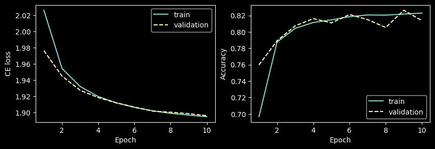
Learning curves
[121]:
fig, axs = plt.subplots(1, 2, figsize=(10, 3))

axs[0].plot(range(1, n_epochs + 1), train_epochs_losses, label='train')
axs[0].plot(range(1, n_epochs + 1), val_epochs_losses, linestyle='dashed', label='validation')

axs[1].plot(range(1, n_epochs + 1), train_epochs_acc, label='train')
axs[1].plot(range(1, n_epochs + 1), val_epochs_acc, linestyle='dashed', label='validation')

axs[0].set_ylabel(loss_func_name)
axs[0].set_xlabel('Epoch')
axs[0].legend()

axs[1].set_ylabel('Accuracy')
axs[1].set_xlabel('Epoch')
axs[1].legend()

plt.show()
[122]:
# array with all losses
# TODO: make with PANDAS?
all_lasses_header = ','.join([
    f'{loss_func_name.split()[0]}_train', f'{loss_func_name.split()[0]}_val',
    'accuracy_train', 'accuracy_val'
])
all_losses_array = np.array(
    [train_epochs_losses, val_epochs_losses, train_epochs_acc, val_epochs_acc]
).T
[ ]:
[ ]:
Saving
[123]:
RESULTS_FOLDER
[123]:
'models/03_mnist_experiments/13-12-2024_experiment_01'
[124]:
if not os.path.exists(RESULTS_FOLDER):
    os.makedirs(RESULTS_FOLDER)
[125]:
# filepath to save the model
model_filepath = f'{RESULTS_FOLDER}/optical_setup_net.pth'
# filepath to save losses
losses_filepath = f'{RESULTS_FOLDER}/training_curves.csv'
[126]:
# saving model
torch.save(lin_optical_setup.net.state_dict(), model_filepath)
[127]:
# saving losses
np.savetxt(
    losses_filepath, all_losses_array,
    delimiter=',', header=all_lasses_header, comments=""
)
[ ]:
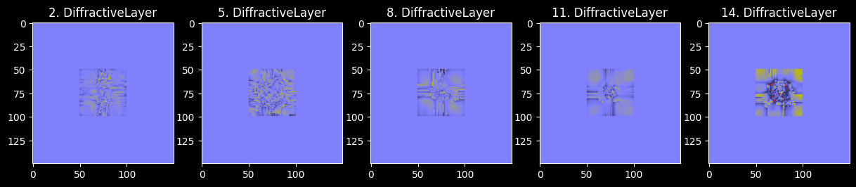
4.2.3. Trained masks
[128]:
n_cols = NUM_OF_DIFF_LAYERS  # number of columns for DiffractiveLayer's masks visualization
n_rows = 1

# plot wavefronts phase
fig, axs = plt.subplots(n_rows, n_cols, figsize=(n_cols * 3, n_rows * 3.2))
ind_diff_layer = 0

cmap = 'gist_stern'

for ind_layer, layer in enumerate(lin_optical_setup.net):
    if isinstance(layer, elements.DiffractiveLayer):  # plot masks for Diffractive layers
        if n_rows > 1:
            ax_this = axs[ind_diff_layer // n_cols][ind_diff_layer % n_cols]
        else:
            ax_this = axs[ind_diff_layer % n_cols]

        ax_this.set_title(f'{ind_layer}. DiffractiveLayer')

        trained_mask = layer.mask.detach()

        # mask_seed = MASKS_SEEDS[ind_diff_layer].item()
        # random_mask = torch.rand(
        #     size=(sim_params.y_nodes, sim_params.x_nodes),
        #     generator=torch.Generator().manual_seed(mask_seed)
        # ) * (MAX_PHASE)

        ax_this.imshow(
            trained_mask, cmap=cmap,
            vmin=0, vmax=MAX_PHASE
        )
        ind_diff_layer += 1

plt.show()
[ ]:
4.2.4. Applying the model to an unknown data (test)
[129]:
# list of all saved models
dir_models = 'models/03_mnist_experiments'

filepathes = []

for file in os.listdir(dir_models):
    filename = os.fsdecode(file)
    if not filename.endswith(".pth"):
        filepathes.append(filename)

print(*sorted(filepathes), sep='\n')
.DS_Store
09-12-2024_experiment_01
13-12-2024_experiment_01
22-11-2024_experiment_01
22-11-2024_experiment_02
22-11-2024_experiment_03
27-11-2024_experiment_01
[130]:
# filepath to save the model
load_model_subfolder = f'13-12-2024_experiment_{EXP_NUMBER:02d}'
load_model_filepath = f'{dir_models}/{load_model_subfolder}/optical_setup_net.pth'

load_model_filepath
[130]:
'models/03_mnist_experiments/13-12-2024_experiment_01/optical_setup_net.pth'
[131]:
# experiment conditions
json.load(open(f'{RESULTS_FOLDER}/conditions.json'))
[131]:
{'wavelength': 0.000749481145,
 'layer_size_m': 0.12,
 'layer_nodes': 150,
 'tensorboard': True,
 'digit_resize': 17,
 'ds_apertures': True,
 'ds_modulation': None,
 'gauss_waist_radius': 0.02,
 'distance_to_aperture': 0.03,
 'propagator': 'AS',
 'n_diff_layers': 5,
 'diff_layer_max_phase': 3.141592653589793,
 'diff_layer_mask_init': 'const',
 'diff_layers_seeds': 123,
 'layers_distance': 0.03,
 'add_apertures': True,
 'apertures_size': [50, 50],
 'detector_zones': 'segments',
 'detector_transpose': False,
 'train_bs': 8,
 'val_bs': 20,
 'train_split_seed': 178,
 'epochs': 10}
[132]:
# setup to load weights
optical_setup_loaded = get_setup(
    SIM_PARAMS,
    NUM_OF_DIFF_LAYERS,
    apertures=ADD_APERTURES,
    aperture_size=APERTURE_SZ
)

# LOAD WEIGHTS
optical_setup_loaded.net.load_state_dict(torch.load(load_model_filepath))
/var/folders/mt/0w6nmsr119bb2g4h4xrv9p6m0000gn/T/ipykernel_98211/3316892598.py:10: FutureWarning: You are using `torch.load` with `weights_only=False` (the current default value), which uses the default pickle module implicitly. It is possible to construct malicious pickle data which will execute arbitrary code during unpickling (See https://github.com/pytorch/pytorch/blob/main/SECURITY.md#untrusted-models for more details). In a future release, the default value for `weights_only` will be flipped to `True`. This limits the functions that could be executed during unpickling. Arbitrary objects will no longer be allowed to be loaded via this mode unless they are explicitly allowlisted by the user via `torch.serialization.add_safe_globals`. We recommend you start setting `weights_only=True` for any use case where you don't have full control of the loaded file. Please open an issue on GitHub for any issues related to this experimental feature.
  optical_setup_loaded.net.load_state_dict(torch.load(load_model_filepath))
[132]:
<All keys matched successfully>
[ ]:
[133]:
test_losses_1, _, test_accuracy_1 = onn_validate_clf(
    optical_setup_loaded.net,  # optical network with loaded weights
    test_wf_loader,  # dataloader of training set
    detector_processor,  # detector processor
    loss_func_clf,
    device=DEVICE,
    show_process=True,
)  # evaluate the model

print(
    'Results after training on TEST set:\n' +
    f'\t{loss_func_name} : {np.mean(test_losses_1):.6f}\n' +
    f'\tAccuracy : {(test_accuracy_1 * 100):>0.1f} %'
)
validation: 100%|████████████████████████████████████████████████████████████████████████| 1000/1000 [00:32<00:00, 30.32it/s]
Results after training on TEST set:
        CE loss : 1.889739
        Accuracy : 82.3 %
[ ]:
4.2.5. Example of classification for a random wavefront (propagation through)
[134]:
# plot an image
# '1' - 3214, good (1318, )
# '4' - 6152, good (1985, )
# '5' - (5134, )
# '6' - 123, good
# '8' - 128, good (1124, 8105)
# '0' - 3, good
ind_test = 6152
cmap = 'hot'

fig, axs = plt.subplots(1, 2, figsize=(2 * 3, 3))

test_wavefront, test_target = mnist_wf_test_ds[ind_test]

axs[0].set_title(f'intensity (id={ind_test})')
axs[0].imshow(test_wavefront.intensity[0], cmap=cmap)

axs[1].set_title(f'phase')
axs[1].imshow(
    test_wavefront.phase[0], cmap=cmap,
    vmin=0, vmax=2 * torch.pi
)

plt.show()
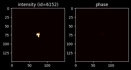
[135]:
test_target
[135]:
4
[136]:
# propagation of the example through the trained network
setup_scheme, test_wavefronts = optical_setup_loaded.stepwise_forward(test_wavefront)
[ ]:
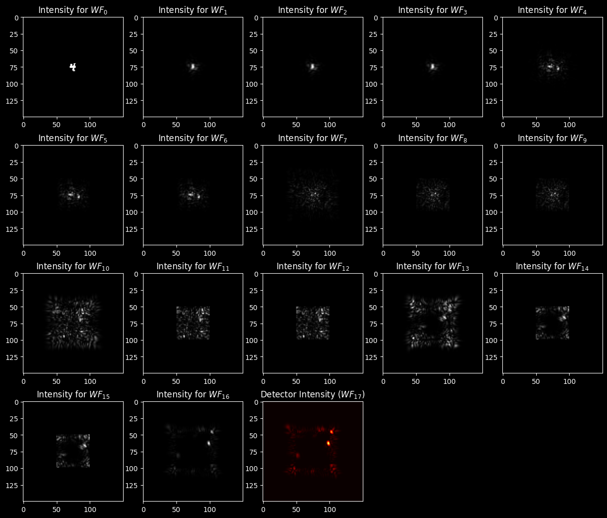
[137]:
print(setup_scheme)  # prints propagation scheme

n_cols = 5  # number of columns to plot all wavefronts during propagation
n_rows = (len(optical_setup_loaded.net) // n_cols) + 1

to_plot = 'amp'  # <--- chose what to plot
cmap = 'grey'  # choose colormaps
detector_cmap = 'hot'

# create a figure with subplots
fig, axs = plt.subplots(n_rows, n_cols, figsize=(n_cols * 3, n_rows * 3.2))

# turn off unecessary axes
for ind_row in range(n_rows):
    for ind_col in range(n_cols):
        ax_this = axs[ind_row][ind_col]
        if ind_row * n_cols + ind_col >= len(wavefronts):
            ax_this.axis('off')

# plot wavefronts
for ind_wf, wavefront in enumerate(test_wavefronts):
    ax_this = axs[ind_wf // n_cols][ind_wf % n_cols]

    if to_plot == 'phase':
        # plot angle for each wavefront, because intensities pictures are indistinguishable from each other
        if ind_wf < len(wavefronts) - 1:
            ax_this.set_title('Phase for $WF_{' + f'{ind_wf}' + '}$')
            ax_this.imshow(
                wavefront[0].phase.detach().numpy(), cmap=cmap,
                vmin=0, vmax=2 * torch.pi
            )
        else:  # (not a wavefront!)
            ax_this.set_title('Detector phase ($WF_{' + f'{ind_wf}' + '})$')
            # Detector has no phase!

    if to_plot == 'amp':
        # plot angle for each wavefront, because intensities pictures are indistinguishable from each other
        if ind_wf < len(wavefronts) - 1:
            ax_this.set_title('Intensity for $WF_{' + f'{ind_wf}' + '}$')
            ax_this.imshow(
                wavefront[0].intensity.detach().numpy(), cmap=cmap,
                # vmin=0, vmax=max_intensity  # uncomment to make the same limits
            )
        else:  # Detector output (not a wavefront!)
            ax_this.set_title('Detector Intensity ($WF_{' + f'{ind_wf}' + '})$')
            ax_this.imshow(
                wavefront[0].detach().numpy(), cmap=detector_cmap,
                # vmin=0, vmax=max_intensity  # uncomment to make the same limits
            )

    # Comment: Detector output is Tensor! It has no methods of Wavefront (like .phase or .intensity)!

plt.show()
-(0)-> [1. FreeSpace] -(1)-> [2. Aperture] -(2)-> [3. DiffractiveLayer] -(3)-> [4. FreeSpace] -(4)-> [5. Aperture] -(5)-> [6. DiffractiveLayer] -(6)-> [7. FreeSpace] -(7)-> [8. Aperture] -(8)-> [9. DiffractiveLayer] -(9)-> [10. FreeSpace] -(10)-> [11. Aperture] -(11)-> [12. DiffractiveLayer] -(12)-> [13. FreeSpace] -(13)-> [14. Aperture] -(14)-> [15. DiffractiveLayer] -(15)-> [16. FreeSpace] -(16)-> [17. Detector] -(17)->
[138]:
# create a figure with subplots
fig, ax_this = plt.subplots(1, 1, figsize=(3, 3.2))

# Detector output (not a wavefront!)
ax_this.set_title('Detector Intensity ($WF_{' + f'{ind_wf}' + '})$')
ax_this.imshow(
    test_wavefronts[-1][0].detach().numpy(), cmap='hot',
    # vmin=0, vmax=1  # uncomment to make the same limits
)

for zone in get_zones_patches(selected_detector_mask):
    # add zone's patches to the axis
    # zone_copy = copy(zone)
    ax_this.add_patch(zone)

plt.show()
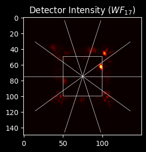
[139]:
# get probabilities of an example classification
test_probas = detector_processor.forward(test_wavefronts[-1])

for label, prob in enumerate(test_probas[0]):
    print(f'{label} : {prob * 100:.2f}%')
0 : 0.85%
1 : 4.22%
2 : 5.14%
3 : 1.11%
4 : 64.29%
5 : 2.39%
6 : 1.11%
7 : 1.32%
8 : 0.70%
9 : 18.87%
[ ]:
[ ]:
[ ]: