[1]:

import torch
import matplotlib.pyplot as plt

from svetlanna import elements
from svetlanna import SimulationParameters
from svetlanna import wavefront as w
from svetlanna.units import ureg

Diffraction on the apertures

We will calculate the diffraction of the plane wave on the different apertures using classes from svetlanna.elements

Creating numerical mesh with using `SimulationParameters` class

[14]:

# screen size
lx = 8 * ureg.mm
ly = 8 * ureg.mm

# distance between the screen and the aperture, mm
z = 220 * ureg.mm

# wavelength, mm
wavelength = 1064 * ureg.nm

# number of nodes
Nx = 1024
Ny = 1024

# creating SimulationParameters exemplar
sim_params = SimulationParameters({
    'W': torch.linspace(-lx / 2, lx / 2, Nx),
    'H': torch.linspace(-ly / 2, ly / 2, Ny),
    'wavelength': wavelength,
})

[15]:

# return 2d-tensors of x and y coordinates
x_grid, y_grid = sim_params.meshgrid(x_axis='W', y_axis='H')

Creating a plane wave using `svetlanna.wavefront.plane_wave`

Let’s create a plane wave that will fall on the aperture:

[16]:

# create plane wave
incident_field = w.Wavefront.plane_wave(
    simulation_parameters=sim_params,
    distance=0 * ureg.cm,
    wave_direction=[0, 0, 1]
)

Creating round aperture using `svetlanna.elements.RoundAperture`

[17]:

radius = 1 * ureg.mm

round_aperture = elements.RoundAperture(
    simulation_parameters=sim_params,
    radius=radius,
)

Let’s see the shape of the aperture using .get_transmission_function() class method:

[18]:

aperture_transmission_function = round_aperture.get_transmission_function()

[19]:

fig, ax = plt.subplots(figsize=(6, 3), edgecolor='black', linewidth=3,
                       frameon=True)
im1 = ax.pcolormesh(x_grid, y_grid, aperture_transmission_function, cmap='inferno')
ax.set_aspect('equal')
ax.set_title('Square aperture shape')
ax.set_xlabel('$x$ [m]')
ax.set_ylabel('$y$ [m]')
fig.colorbar(im1, label='Transmission function')

[19]:

<matplotlib.colorbar.Colorbar at 0x12fcb746a90>

../../_images/examples_notebook_freeprop_apertures_11_1.png

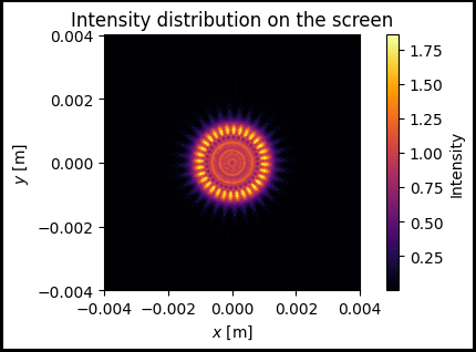
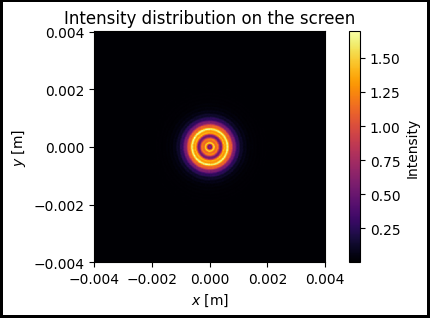
Intensity profile on the screen after propagation through the round aperture

In this section we will solve the direct problem of diffraction on a round aperture using Angular Spectrum method from FreeSpace class

[20]:

field_after_aperture = round_aperture.forward(
    incident_wavefront=incident_field
)

free_space = elements.FreeSpace(
    simulation_parameters=sim_params,
    distance=z,
    method="AS"
)

output_wavefront = free_space.forward(
    incident_wavefront=field_after_aperture
)

output_intensity = output_wavefront.intensity

Visualize the intensity distribution:

[21]:

fig, ax = plt.subplots(figsize=(6, 3), edgecolor='black', linewidth=3,
                       frameon=True)
im1 = ax.pcolormesh(x_grid, y_grid, output_intensity, cmap='inferno')
ax.set_aspect('equal')
ax.set_title('Intensity distribution on the screen')
ax.set_xlabel('$x$ [m]')
ax.set_ylabel('$y$ [m]')
fig.colorbar(im1, label='Intensity')

[21]:

<matplotlib.colorbar.Colorbar at 0x12fcbc1f110>

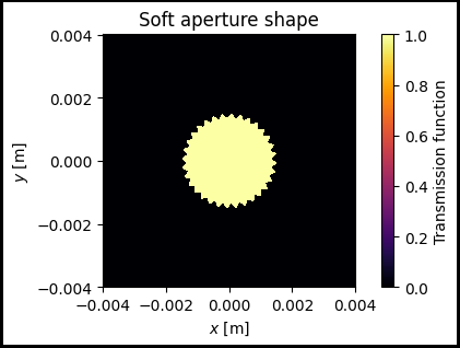
Creating aperture with arbitrary shape

For the instance, we will create the aperture which is similar to the soft aperture from the article [1]

The shape of the aperture is determined by the expression:

\[r=R + S(\theta)=R(1 + \dfrac{s}{2}(1 + \sin{M\theta})),\]

where \(R\) - radius of the round aperture, \(M\) - number of serrations, \(s\) - is the ratio of the serrated height \(h\) to \(r\).

Let’s create the shape of the aperture:

[42]:

radius_soft = 1 * ureg.mm

r = torch.sqrt(x_grid**2 + y_grid**2)
M = 32

s = 0.1

theta = torch.atan2(y_grid, x_grid)
shape = r *( 1 + s / 2 *(1 + torch.sin(M*theta)))
shape = shape < 0.0015

Creating aperture with determined shape using Aperture class from the svetlanna.elements

[43]:

soft_aperture = elements.Aperture(simulation_parameters=sim_params, mask=shape)

Let’s see the shape of the soft aperture using .get_transmission_function() class method:

[44]:

aperture_transmission_function = soft_aperture.get_transmission_function()

[46]:

fig, ax = plt.subplots(figsize=(6, 3), edgecolor='black', linewidth=3,
                       frameon=True)
im1 = ax.pcolormesh(x_grid, y_grid, aperture_transmission_function, cmap='inferno')
ax.set_aspect('equal')
ax.set_title('Soft aperture shape')
ax.set_xlabel('$x$ [m]')
ax.set_ylabel('$y$ [m]')
fig.colorbar(im1, label='Transmission function')

[46]:

<matplotlib.colorbar.Colorbar at 0x12f8eddfd50>

../../_images/examples_notebook_freeprop_apertures_23_1.png

Intensity profile on the screen after propagation through the soft aperture

In this section we will solve the direct problem of diffraction on a soft aperture using Angular Spectrum method from FreeSpace class

[47]:

field_after_aperture = soft_aperture.forward(
    incident_wavefront=incident_field
)

free_space = elements.FreeSpace(
    simulation_parameters=sim_params,
    distance=z,
    method="AS"
)

output_wavefront = free_space.forward(
    incident_wavefront=field_after_aperture
)

output_intensity = output_wavefront.intensity