Lens

import torch
import matplotlib.pyplot as plt

from svetlanna import elements
from svetlanna import SimulationParameters
from svetlanna import wavefront as w
from svetlanna.units import ureg
from svetlanna import LinearOpticalSetup

from PIL import Image

Creating numerical mesh with using SimulationParameters class

# screen size
lx = 8 * ureg.mm
ly = 8 * ureg.mm

# focal length, mm
f = 100 * ureg.mm

# wavelength, mm
wavelength = 1064 * ureg.nm

# number of nodes
Nx = 2048
Ny = 2048

# creating SimulationParameters exemplar
sim_params = SimulationParameters({
    'W': torch.linspace(-lx / 2, lx / 2, Nx),
    'H': torch.linspace(-ly / 2, ly / 2, Ny),
    'wavelength': wavelength,
})

# return 2d-tensors of x and y coordinates
x_grid, y_grid = sim_params.meshgrid(x_axis='W', y_axis='H')

Creating a plane wave using svetlanna.wavefront.plane_wave

Let’s create a plane wave that will fall on the aperture:

# create plane wave
incident_field = w.Wavefront.plane_wave(
    simulation_parameters=sim_params,
    distance=10 * ureg.cm,
    wave_direction=[0, 0, 1]
)

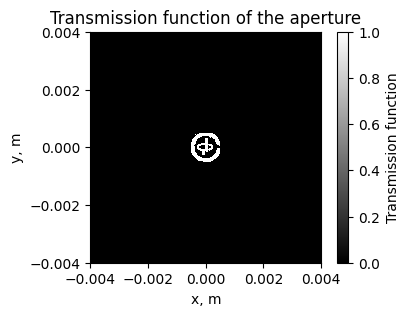
Prepare image: converting to mask for the aperture

In this section we convert the image phystech_logo.png to aperture. The shape of the aperture will match the image.

# path to the image
image_path = '.\doc\phystech_logo.png'  # Замените на путь к вашему изображению

# image size
N, M = 256, 256

# Загрузка изображения
image = Image.open(image_path)

M = 256
# change image size
image_resized = image.resize((N, M))  # Размеры указываются как (ширина, высота)

# convert image to tensor
image_tensor = torch.tensor(
    data=list(image_resized.getdata()),
    dtype=torch.float64
).reshape(N, M, -1)

# normalize image tensor to [0, 1] range
if image_tensor.dtype == torch.uint8:
    image_tensor = image_tensor / 255.0

# use only one channel of the image (grayscale)
image_tensor = image_tensor[:, :, 0]

# binarize the image tensor
image_tensor = image_tensor >= 10  # Применяем бинаризацию

# Определяем координаты для вставки image_tensor в центр mask
start_x = (Nx - M) // 2
start_y = (Ny - N) // 2

mask = torch.zeros((Ny, Nx), dtype=torch.float64)

# put image_tensor in the center of the mask
mask[start_y:start_y + N, start_x:start_x + M] = image_tensor

aperture = elements.Aperture(simulation_parameters=sim_params, mask=mask)

fig, ax = plt.subplots(figsize=(4, 3))

im = ax.pcolormesh(x_grid, y_grid, aperture.get_transmission_function(), cmap='gray')
ax.set_aspect('equal')
ax.set_xlabel('x, m')
ax.set_ylabel('y, m')
ax.set_title('Transmission function of the aperture')
fig.colorbar(im, ax=ax, label='Transmission function')

<matplotlib.colorbar.Colorbar at 0x10a0ffee790>

Creating optical setup

In this section we create optical setup using LinearOpticalSetup class from svetlanna.setup. Optical setup consists of aperture with transmission function determined by mask tensor and thin collecting lens. Wavefront propagation calculated by FreeSpace element using Angular Spectrum method.

lens = elements.ThinLens(
    simulation_parameters=sim_params,
    focal_length=f,
    radius=100 * ureg.mm
)

free_space = elements.FreeSpace(
    simulation_parameters=sim_params,
    distance=f,
    method="AS"
)

setup = LinearOpticalSetup([aperture, free_space, lens, free_space])

Calculating the wavefront in the back focal plane of the thin lens

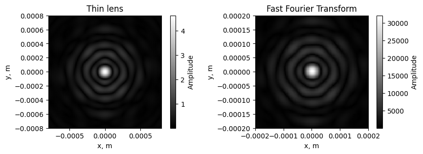
As is known, a thin lens performs a Fourier transform from a wavefront incident on it. Let’s compare the Fourier image created by the thin lens and Fourier image created by the Fast Fourier Transform from torch.fft.fft2.

output_wavefront = setup.forward(input_wavefront=incident_field)
output_intensity = output_wavefront.intensity

fft = torch.fft.fftshift(torch.fft.fft2(mask))

fig, ax = plt.subplots(1, 2, figsize=(10, 3))
im0 = ax[0].pcolormesh(x_grid, y_grid, torch.sqrt(output_intensity), cmap='gray')
ax[0].set_aspect('equal')
ax[0].set_xlabel('x, m')
ax[0].set_ylabel('y, m')

ax[0].set_xlim(-lx / 10, lx / 10)
ax[0].set_ylim(-ly / 10, ly / 10)
ax[0].set_title('Thin lens')
fig.colorbar(im0, ax=ax[0], label='Amplitude')

im1 = ax[1].pcolormesh(x_grid, y_grid, torch.abs(fft), cmap='gray')
ax[1].set_aspect('equal')
ax[1].set_xlabel('x, m')
ax[1].set_ylabel('y, m')

ax[1].set_xlim(-lx / 40, lx / 40)
ax[1].set_ylim(-ly / 40, ly / 40)
ax[1].set_title('Fast Fourier Transform')
fig.colorbar(im1, ax=ax[1], label='Amplitude')

<matplotlib.colorbar.Colorbar at 0x10a1943e650>