import torch
import matplotlib.pyplot as plt

from svetlanna import elements
from svetlanna import SimulationParameters
from svetlanna import wavefront as w
from svetlanna.units import ureg

import analytical_solutions as anso

Propagation through the square aperture

In this example we will use rectangular aperture from svetlanna.elements to solve the diffraction problem.

Creating numerical mesh with using SimulationParameters class

# screen size
lx = 4 * ureg.mm
ly = 4 * ureg.mm

# distance between the screen and the aperture, mm
z = 220 * ureg.mm

# size of the aperture, mm
a = 1 * ureg.mm

# wavelength, mm
wavelength = 1064 * ureg.nm

# number of nodes
Nx = 2048
Ny = 2048

# creating SimulationParameters exemplar
sim_params = SimulationParameters({
    'W': torch.linspace(-lx / 2, lx / 2, Nx),
    'H': torch.linspace(-ly / 2, ly / 2, Ny),
    'wavelength': wavelength,
})

# return 2d-tensors of x and y coordinates
x_grid, y_grid = sim_params.meshgrid(x_axis='W', y_axis='H')

Creating a plane wave using svetlanna.wavefront.plane_wave

Let’s create a plane wave that will fall on the aperture:

# create plane wave
incident_field = w.Wavefront.plane_wave(
    simulation_parameters=sim_params,
    distance=0 * ureg.cm,
    wave_direction=[0, 0, 1]
)

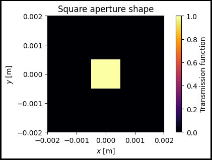
Creating a square aperture using svetlanna.elements.RectangularAperture

square_aperture = elements.RectangularAperture(
    simulation_parameters=sim_params,
    height=a,
    width=a,
)

Let’s see the shape of the aperture using .get_transmission_function() class method:

aperture_transmission_function = square_aperture.get_transmission_function()

fig, ax = plt.subplots(figsize=(6, 3), edgecolor='black', linewidth=3,
                       frameon=True)
im1 = ax.pcolormesh(x_grid, y_grid, aperture_transmission_function, cmap='inferno')
ax.set_aspect('equal')
ax.set_title('Square aperture shape')
ax.set_xlabel('$x$ [m]')
ax.set_ylabel('$y$ [m]')
fig.colorbar(im1, label='Transmission function')

<matplotlib.colorbar.Colorbar at 0x1a3f5428310>

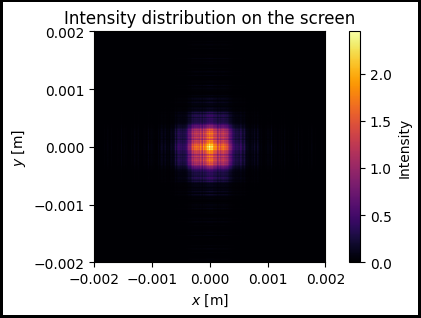
Intensity profile on the screen after propagation through the square aperture

In this section we will solve the direct problem of diffraction on a square aperture using Angular Spectrum method from FreeSpace class

field_after_aperture = square_aperture.forward(
    incident_wavefront=incident_field
)

free_space = elements.FreeSpace(
    simulation_parameters=sim_params,
    distance=z,
    method="AS"
)

output_wavefront = free_space.forward(
    incident_wavefront=field_after_aperture
)

output_intensity = output_wavefront.intensity

Visualize the intensity distribution:

fig, ax = plt.subplots(figsize=(6, 3), edgecolor='black', linewidth=3,
                       frameon=True)
im1 = ax.pcolormesh(x_grid, y_grid, output_intensity, cmap='inferno')
ax.set_aspect('equal')
ax.set_title('Intensity distribution on the screen')
ax.set_xlabel('$x$ [m]')
ax.set_ylabel('$y$ [m]')
fig.colorbar(im1, label='Intensity')

<matplotlib.colorbar.Colorbar at 0x1a3f5203c50>

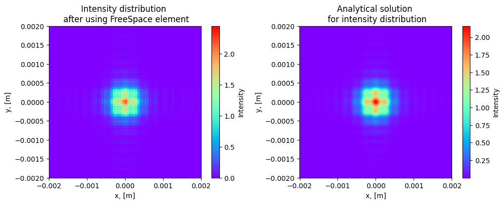
Comparing with analytical solution

In this section we wll compare our numeric solution which was calculated using Angular Spectrum method with analytical solution of the problem that expressed in terms of Fresnel’s integrals

rect_int = anso.SquareFresnel(
    distance=z,
    x_size=lx,
    y_size=ly,
    x_nodes=Nx,
    y_nodes=Ny,
    square_size=a,
    wavelength=wavelength
)

intensity_analytic = rect_int.intensity()

Let’s visualize both intensity distributions:

fig, ax = plt.subplots(1, 2, figsize=(12, 4))
beam1 = ax[0].pcolormesh(x_grid, y_grid, output_intensity, cmap='rainbow')
beam2 = ax[1].pcolormesh(x_grid, y_grid, intensity_analytic, cmap='rainbow')

ax[0].set_title('Intensity distribution \n after using FreeSpace element')
ax[1].set_title('Analytical solution \n for intensity distribution')

ax[0].set_aspect('equal')
ax[1].set_aspect('equal')

ax[0].set_xlabel('x, [m]')
ax[0].set_ylabel('y, [m]')
ax[1].set_xlabel('x, [m]')
ax[1].set_ylabel('y, [m]')
fig.colorbar(beam1, ax=ax[0], label='Intensity')
fig.colorbar(beam2, ax=ax[1], label='Intensity')

<matplotlib.colorbar.Colorbar at 0x1a41a81a8d0>