import torch
import numpy as np
import matplotlib.pyplot as plt

from svetlanna import elements
from svetlanna import SimulationParameters
from svetlanna import wavefront as w
from svetlanna.units import ureg

Diffraction on the thin slit

We will calculate the diffraction of the plane wave on the thin slit using rectangular aperture from svetlanna.elements

Creating numerical mesh with using SimulationParameters class

D = 0.1 * ureg.mm   # width of the slit
d = 0.5 * ureg.mm   # height of the slit

wavelength = 660 * ureg.nm  # wavelength

lx = 4 * ureg.mm  # width of the screen
ly = 4 * ureg.mm  # height of the screen

# distance from the slit to the screen
z = 3 * ureg.cm

# number of nodes along x and y
Nx = 1600
Ny = 1600

# creating SimulationParameters exemplar
sim_params = SimulationParameters({
    'W': torch.linspace(-lx / 2, lx / 2, Nx),
    'H': torch.linspace(-ly / 2, ly / 2, Ny),
    'wavelength': wavelength,
})

# return 2d-tensors of x and y coordinates
x_grid, y_grid = sim_params.meshgrid(x_axis='W', y_axis='H')

Creating a plane wave using svetlanna.wavefront.plane_wave

Let’s create a plane wave that will fall on the aperture:

# create plane wave
incident_field = w.Wavefront.plane_wave(
    simulation_parameters=sim_params,
    distance=0 * ureg.cm,
    wave_direction=[0, 0, 1]
)

Creating a thin slit using svetlanna.elements.RectangularAperture

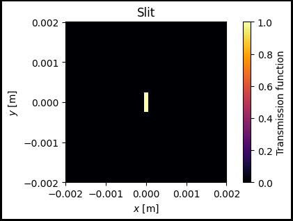
slit = elements.RectangularAperture(
    simulation_parameters=sim_params,
    height=d,
    width=D,
)

Let’s see the shape of the aperture using .get_transmission_function() class method:

slit_transmission_function = slit.get_transmission_function()

fig, ax = plt.subplots(figsize=(6, 3), edgecolor='black', linewidth=3,
                       frameon=True)
im1 = ax.pcolormesh(x_grid, y_grid, slit_transmission_function, cmap='inferno')
ax.set_aspect('equal')
ax.set_title('Slit')
ax.set_xlabel('$x$ [m]')
ax.set_ylabel('$y$ [m]')
fig.colorbar(im1, label='Transmission function')

<matplotlib.colorbar.Colorbar at 0x218e8fc2c50>

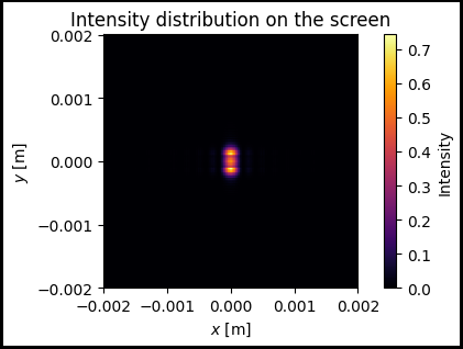
Intensity profile on the screen after propagation through the slit

In this section we will solve the direct problem of diffraction on a slit using Angular Spectrum method from FreeSpace class

field_after_slit = slit.forward(
    incident_wavefront=incident_field
)

free_space = elements.FreeSpace(
    simulation_parameters=sim_params,
    distance=z,
    method="AS"
)

output_wavefront = free_space.forward(
    incident_wavefront=field_after_slit
)

output_intensity = output_wavefront.intensity

Visualize the intensity distribution:

fig, ax = plt.subplots(figsize=(6, 3), edgecolor='black', linewidth=3,
                       frameon=True)
im1 = ax.pcolormesh(x_grid, y_grid, output_intensity, cmap='inferno')
ax.set_aspect('equal')
ax.set_title('Intensity distribution on the screen')
ax.set_xlabel('$x$ [m]')
ax.set_ylabel('$y$ [m]')
fig.colorbar(im1, label='Intensity')

<matplotlib.colorbar.Colorbar at 0x218ec697e50>

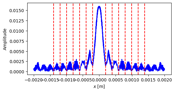
Comparing with diffraction grating equation

Using the diffraction grating equation \(D \sin{\theta}=m\lambda\), where m is the order of diffraction, we can find the position of the intensity minima:

# array of min
m  = np.arange(1,8,1)
x_min = np.sqrt(m**2 * wavelength**2 * z**2 / (D**2 - m**2 * wavelength**2))

fig, ax = plt.subplots(figsize=(6, 3))
ax.plot(x_grid[0], torch.sqrt(output_intensity)[250], color='blue')

[ax.axvline(x, ls='--', color='r') for x in x_min]
[ax.axvline(-x, ls='--', color='r') for x in x_min]

ax.set_xlabel('$x$ [m]')
ax.set_ylabel('Amplitude')

Text(0, 0.5, 'Amplitude')